Why cDNA?
Our example data: Large-scale temporal gene expression mapping of CNS development
Link to the raw data
and PDF.
Reference: Wen X, Fuhrman S, Michaels GS, Carr DB, Smith S, Barker JL, Somogyi R (1998)
Large-Scale Temporal Gene Expression Mapping of CNS Development.
Proc Natl Acad Sci USA, 95:334-339.
Abstract: Examine gene function by looking for expression patterns that correlate with rat CNS developmental stages. Samples are 9 stages: embryonic (E11-21 days), post-natal (P0-P14), and adult (P90). Variables are 112 gene expression levels measured by RT-PCR.
The raw data from Somogyi's paper is available. For convenience, I have pre-parsed data using a perl parser that is also available.
As you go to different sites, you'll notice that each has its own format for saving information. You have to write an individual parser for each. Wouldn't it be nice to have a central repository for gene expression information in a standardized format that allowed you to make direct comparisons between different data sets? (See suggested projects.) The EBI has issued a press release stating their desire to do just this.
Simple idea: find genes that are up- or down-regulated in a particular comparison. Simple solution: sort a list. Quickly find that this information isn't sufficient.
Slightly more complex idea:
What is a good measure of expression profile similarity? Can we define a distance so that genes with similar profiles have a smaller distance, genes with different profiles have a larger distance? Think about how we measure sequence similarity: one way is to count the number of indels and subs to get a score.
Suppose we have genes A and B and look at several biological states numbered 1, 2, 3, ..., N:
| Gene | State 1 | State 2 | ... | State N |
|---|---|---|---|---|
| A | A1 | A2 | ... | AN |
| B | B1 | B2 | ... | BN |
A1, A2, ... are numbers that tell us the expression level in some units (flourescence intensity, # of sequences in an EST database, intensity relative to some control, ...).
There are many ways to define a distance. A good reference is Multivariate Analysis by Mardia, Kent, and Bibby. Here are some typical choices to get D(A,B) between genes A and B.
| Method | Formula | Good points | Bad points |
|---|---|---|---|
| Euclidean distance | D(A,B) = Sum (Ai - Bi)2, i = 1 .. N |
Easy to calculate | Two genes that have exactly the same shape to their expression profiles but differ in amplitude can end up far apart. Genes with different profiles but that are both expressed at low levels can end up close together. |
| Pearson correlation coefficient distance | corln coef C = [Sum AiBi - (1/N) Sum Ai Sum Bi] / [SA SB] SA = sqrt[Sum Ai2 - (1/N) (Sum Ai)2] SB = sqrt[Sum Bi2 - (1/N) (Sum Bi)2] Then D(A,B) = sqrt(2 - 2 C) |
The correlation coefficient is a useful statistical measure. People will know (or at least pretend to know) what you're talking about. It fixes most of the problems with the Euclidean distance measure. | A single large difference in the expression levels of A and B in a particular experiment (or a single bad data point) can dominate the measure, just as an outlier can through off a least squares line. |
| Spearman (rank-order) correlation | Sort the expression values A1, A2, ..., AN, then replace each value by its order in the sorted list. For example, with (A1,A2,A3,A4) = (0.5, 0.7, 0.2, 1.3), the new values would be (A1,A2,A3,A4) = (2, 3, 1, 4). Do the same for the measurements of gene B, then follow the Pearson formulas. | Non-parametric statistics are more robust than parametric statistics. Translation: this reduces the effect of outliers. | Might be less sensitive than Pearson |
Installing PDL
Suppose you wanted to look for similarities between biological states.
One solution would be to take a matrix transpose before calculating the
distances. The software already does this:
perl express.pl t < datafile
and here are the distances. This could be useful
if the biological states are different drugs and you want to see which
have the same mechanism of action.
A matrix of distances doesn't do much good. But you can use it to organize the genes according to similarity. One approach is hierarchical classification. There are simple algorithms that use pairwise distances to generate a branching tree. Here's a typical algorithm called neighbor joining:
I called the output of express.pl infile because that's the file that neighbor_jsb expects to read. Run neighbor_jsb and you get two files:
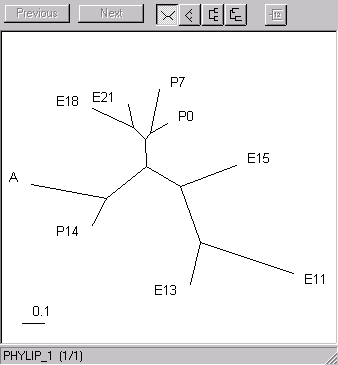
Important point: parentheses are part of the syntax of the treefile and really should be parsed out of sample names. I don't do this yet. You can load the treefile into a viewer like treeview (PCs and Macs only, and it barfs on parentheses). Here are the trees I got for the genes and the samples.| The samples. The early embryonic (11-15 days) branch off, as do the latest stages (14 days postnatal and adult). The late embryonic and early post-natal form a third cluster. | |
| The genes | 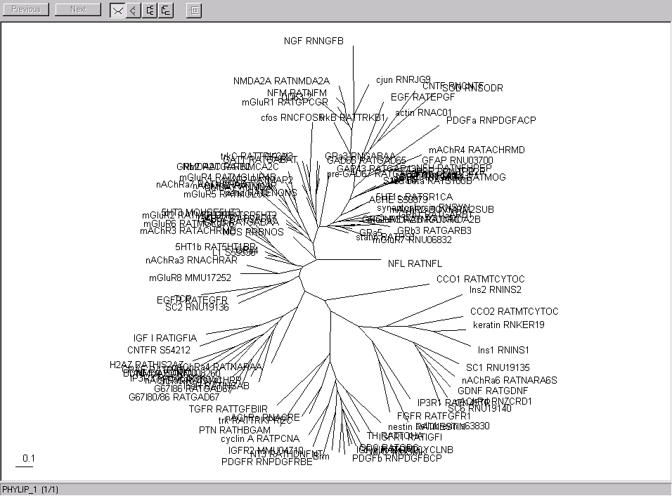 |
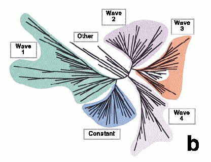
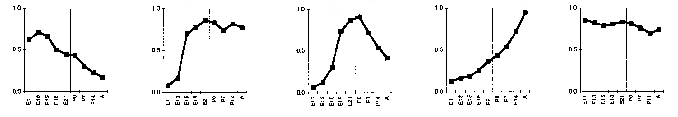
In a case like this, it's easy to define clusters, or waves, by eye. You can modify a hierarchical classification algorithm to build clusters by defining initial groups to contain all genes within a pre-determined distance of each other. In the figure below, also from the Somogyi paper, the temporal profiles are shown separately for each of the clusters.
Suppose that we could really define a set of factors F1, F2, ...
so that the expression level of gene A is
A = L(A,1)F1 + L(A,2)F2 + ...,
the expression level of gene B is
B = L(B,1)F1 + L(B,2)F2 + ...,
and so on. This helps us understand what's going on if the
number of factors we use is smaller than the number of genes.
Also, the factors should end up having something to do with
biological pathways or functional roles.
(In the example we're using, this should be true because
we can see by eye that 4 or 5 pathways describe the main features
of the hierarchical classification.) Mathematically, our goal is
to choose a set of factors F1, F2, ..., and a set of factor loadings
L(A,1), L(A,2), ..., L(B,1), L(B,2), ..., that best explain the data.
The magical recipe is
L(A,i) = U(A,i)sqrt(Ei)
where U(A,i) is the ith eigenvector of the matrix HCH
arranged in decreasing order of eigevalue Ei; C(A,B) is the correlation
between genes A and B calculated from one of the recipes above, or set
to -(1/2)D(A,B) where D is any distance metric, and H is the centering
matrix with diagonal elements 1 - 1/N and off-diagonal elements -1/N
with N the number of genes. When we multiply by the square root,
it's called principal factor analysis. If we stop before the multiplication,
it's called principal component analysis.
To get the principal components describing the genes, run
perl express.pl p < somogyi.txt
and to get the principal components describing the biological states,
perl express.pl tp < somogyi.txt
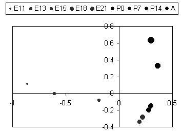
| In this figure the biological states (embryonic days, post-natal days, and adult) are plotted according to the first and second principal factors. The first factor apparantly describes changes during embryonic development culminating at E18, and the second factor describes changes from E18 to Adult. Now we see why E18, E21, P0, and P7 were grouped together in the clustering. |
|